Mercury: A New Curve Primitive For On-chain Token Liquidity

Since the beginning of DeFi, almost every token's on-chain liquidity has been determined by a single liquidity curve, the constant product invariant x*y=K. In my last article New Curve, New Era, I discussed how x*y=K is an ineffective curve for on-chain token liquidity, and why a new curve needs to be specifically designed to serve this use case.

In this article I will introduce Baseline Mercury, explore the mathematical properties behind liquidity curves, and show you why Mercury's invariant is especially suited for on-chain token liquidity. I believe Mercury will enable a new era for native on-chain asset issuance, and by the end of the article, you will too.

Let's begin.

There's No Such Thing as a Perfect Curve

In a vacuum, no liquidity curve is inherently better than another. Saying that is like saying that a screwdriver is better than a hammer: it doesn't make sense because they are useful in different situations and meant to serve different purposes.

The same applies to liquidity curves. When I say that the x*y=K curve is ineffective, I don't mean that there is anything inherently wrong with the equation. I just mean that the specific properties defined by the curve are not useful or desirable for projects that need on-chain liquidity for their tokens.

To understand why, it's necessary to first understand what a liquidity curve is. A curve simply defines a relationship between how the balances of a pool's inventory—its tokens and reserves—change relative to each other across a price spectrum. This can be more intuitively understood from the perspective of an order book: a curve dictates how concentrated orders are at various levels within the book, and how fast the sizes of those orders shrink or grow based on the price.

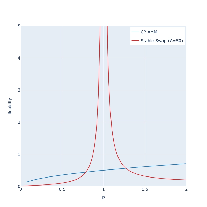
Every curve has different conditions where it performs better or worse than others. A curve that sells tokens conservatively outperforms a curve that sells them aggressively in a market where the token price increases. The same curve underperforms if the price ends up decreasing instead. To visualize this effect, here are three different invariant curves and how they perform in response to the same price changes:

As such, when evaluating curves, it's critical to understand the choices and preferences on inventory implied by the invariant, and more importantly, what market structure and outcomes the curve is intending to optimize for.

The Fallacy of General Purpose

This idea is best illustrated by the stableswap invariant, a specialized curve for stablecoin liquidity. In the stableswap invariant, a large amount of pool reserves and tokens can be exchanged without changing price too much, resulting in the vast majority of its liquidity concentrated around a single point. This makes the stableswap invariant a particularly good curve for tokens who expect to stay $1.00 forever, and horrible for everything else.

For natively issued tokens, the only curve that exists for on-chain liquidity is the constant product invariant x*y=K. This curve ensures that an equal ratio of tokens and reserves is preserved regardless of price movement, providing even liquidity across every conceivable price. Many people conflate the price agnostic property of the curve with the idea that it is a general purpose liquidity solution, but this could not be further from the truth.

As we established in the outset, each curve performs better under a specific scenario, and x*y=K is no exception. Constant product liquidity works well under two conditions: the first is when the liquidity pool is not responsible for price discovery, and the second is when the majority of the liquidity belongs outside of the pool. This makes it a great curve to maintain balanced exposure to assets that have already undergone significant price discovery like ETH or BTC.

However, this makes it a horrible curve for projects deploying their own token liquidity!

The constant product invariant is awful at price discovery because that's not what it's designed to do: the curve is designed to respond to external price changes in order to maintain the balance of its internal inventory, not to determine the fair price of a token based on the ratio of available assets in the pool.

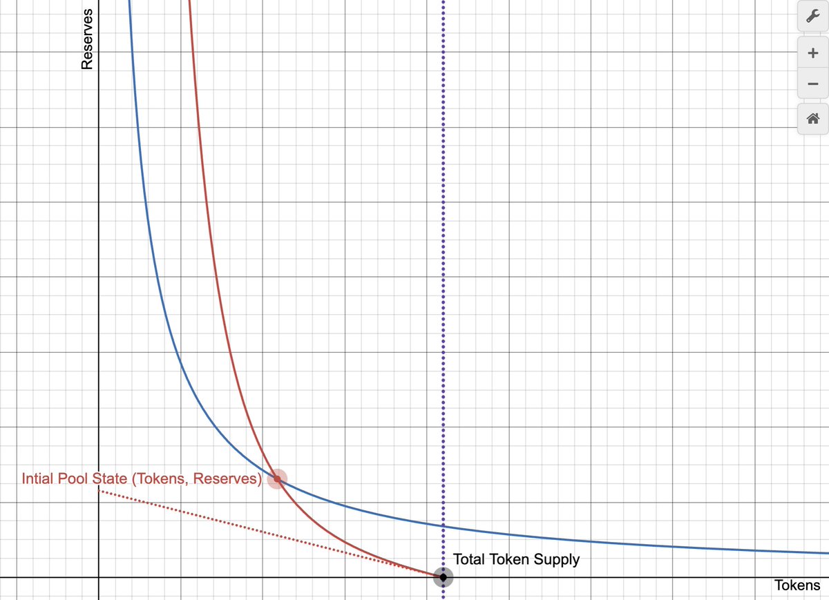
The initial ratio of tokens to reserves deposited in the pool permanently determines price sensitivity, liquidity depth, and supply distribution for all possible future iterations of the pool. A minor difference in this ratio has massive cascading effects for how price changes and liquidity grows at different token market caps as the supply expands and contracts along the curve.

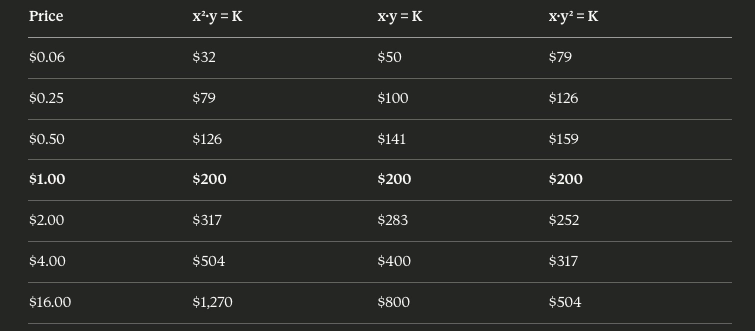
The clearest example of this comes from the fact that the constant product equation breaks when the liquidity pool owns more than half of a token's total supply. Mathematically speaking:

In plain english, this means that when a pool owns more than half the total supply of a token, the TVL of the pool's liquidity becomes more valuable than the entire FDV of the underlying token, violating all financial rationality.

It's how you end up with things like this:

I will never not think about $SLERF. Rent free forever.

Or this:

So now you know how it works!

The Deployer's Demise

The deeper insight is that the x*y=K equation has no concept about a token's supply at all. The invariant is based on the token supply in the pool, not the total supply in existence. That's why the curve has no way to tell a token's market cap: it's literally not part of the equation.

This puts the responsibility of pricing the asset, designing the liquidity profile, and distributing the supply squarely on the deployer. The problem is, as we've already determined, "good liquidity" and "price volatility" at one market cap isn't guaranteed at another. There's no single pool configuration that adapts to all possible future states—it's an impossible task. At some point, these pools will break for one reason or another.

I firmly believe that this is a major reason, if not the primary reason, why crypto so far has been a failed experiment. I believe it's why DeFi "failed", why every launchpad failed, why HIP-2 failed (even Hyperliquid couldn't make it work), why tokens only launch on CEXs, why every chart looks the same, and why everyone who launches a token eventually gets labeled a scammer, grifter, or failure.

The single misconception that this "general purpose" curve is sufficient to deploy on-chain liquidity with has probably set the industry back decades of time and billions of capital.

But in a way it also makes me extremely bullish, because I think if we can fix the curve, we'll fix a lot of things in crypto. That's why, despite watching the industry burn down in a giant dumpster fire over the last few years, despite massive amounts of talent pivoting to AI, and despite the general loss of faith, money and vibes, the team at @BaselineMarkets never really stopped pushing on liquidity innovation.

And finally, after years of development, we finally have something to present: a new curve specially made to solve on-chain liquidity for tokens.

We're calling it Mercury, and it looks like this:

$y = K \cdot (cx)^2 + BLV \cdot c$

Different Assumptions, Different Outcomes

Mercury is an invariant curve designed for the sole purpose of defining a liquidity structure around a token's circulating supply, rather than the internal balances of the pool. The equation uses a new input, c, which represents the total supply of tokens held outside the pool, to establish a proper accounting for liquidity utilization around every possible state of circulation.

By doing so, price scales naturally based on the degree of supply distribution: what makes a token valuable is based on the ratio of tokens that want to be held versus the tokens that have already been dumped. This allows Mercury's curve to provide smoother price discovery and deeper liquidity profile across the entire lifecycle of the token, offering higher capital utilization and efficiency throughout.

This becomes especially relevant when the pool holds a larger portion of the total supply in two ways. First, regardless of how many tokens sit in the liquidity pool, the pool won't feel "too thick". Upward price volatility is not suppressed by a dense token supply in the pool and prevents tokens from being easily acquired from the pool at low prices. This helps prevent against "bundling", or supply cornering, at low points on the curve.

Second, there is no leftover capital when the entire supply is sold into the pool. Mercury knows when there are no more tokens left to buy, and can therefore budget accordingly to ensure it uses all of its available capital to buy out all remaining tokens in circulation. This also allows Mercury to sustain higher prices along all points on the curve, since no idle capital sits in unreachable price ranges.

Another unique thing about the Mercury equation is the value decomposition of each token. Unlike x*y=K, which describes a singular relationship between the two balances of the pool, Mercury's curve is actually two separate pricing curves added together, with each serving a different purpose in the system.

The first price component is a Baseline Value (BLV) for each token in circulation. This value stays the same no matter how many or few tokens are in the market, forming a price support for the market that sets the foundation for its valuation. The second price component is the premium value, which scales quadratically for each additional token in circulation. This describes the additional value on top of the baseline, ensuring price growth as the marginal demand for tokens increases.

Together, this combination supports healthy token price and liquidity for all market conditions. When demand is strong and the overall supply is widely distributed into the market, the token becomes extremely valuable, trading at multiples above its baseline. In periods of lower circulation, the premium compresses and the token trades closer to its BLV. In a full market unwind scenario, the premium drops to zero, and the price of the token returns to its baseline price.

What this means is that project founders and token deployers finally have a liquidity curve that automatically adapts to the appropriate market conditions without needing to worry about initial liquidity configurations. They finally have a liquidity pool that proactively improves itself over time, mathematically optimized to drive long-term value accrual to every single token in circulation. They finally have a liquidity solution that they can view as an asset, rather than a liability.

They finally have a future. And that future begins with Mercury.

To learn more, view our docs.

To see the curves in action yourself, check out the Baseline Simulator: